What is decompilation? The pipeline and the contract

What is Decompilation and Why is it Useful?

Imagine you are working at a company and come across a new ransomware executable that poses a threat to your company. You need to figure out the logic of the ransomware to make the necessary changes to defend against cyber attacks using this new ransomware. However, you do not have access to the source code or any other information about the program.

What is ransomware?

Ransomware is a type of malicious software (malware) that encrypts a victim’s files, devices, or network, rendering them inaccessible. Attackers demand a ransom payment, hence the name "ransom"ware, in exchange for the decryption key to restore access.

Why Not Just Run the Executable?

Running the executable can give a general sense of what a program does, but it rarely tells the whole story. Moreover, when dealing with malware or untrusted software, it may not be safe for us to run the program at all. Running the ransomware executable within the company's environment could lead to the encryption of countless files critical to running the organization.

Analysts mitigate this risk by using sandboxes, isolated environments designed to observe a program's behavior without exposing real systems to the malware. Other safety measures, such as network isolation and virtual machine snapshots, can also contain the effects of the malware. However, a sophisticated piece of malware may detect the presence of a sandbox or virtual environments, suppressing its true functionality and making dynamic analysis unreliable.

From Source Code to Binary

Instead, we can try to inspect the code directly. While it would be optimal to inspect the source code directly, a malicious actor is unlikely to provide us with such luxury. More likely, we could be dealing with just the compiled binary, where much of the high-level structure and semantic information of the original code is lost, leaving machine code that is nearly impossible to understand for humans.

Consider the contrast below:

int fibonacci(int n) {
    if (n <= 1) 
        return n;

    return fibonacci(n - 1) + fibonacci(n - 2);
}

f3 0f 1e fa 55 48 89 e5  53 48 83 ec 18 89 7d ec
83 7d ec 01 7f 05 8b 45  ec eb 1e 8b 45 ec 83 e8
01 89 c7 e8 d8 ff ff ff  89 c3 8b 45 ec 83 e8 02
89 c7 e8 c9 ff ff ff 01  d8 48 8b 5d f8 c9 c3

At a glance, the C source clearly describes a recursive Fibonacci function. The machine code tells the same story, but in a form that is nearly impossible for a human to read or reason about.

Disassembly - A Partial Solution

Disassembly can sometimes offer help, converting machine code into assembly language, making the program more approachable and the instructions at least legible. But for programs with complex algorithms or intricate control flow, assembly still leaves much of underlying logic difficult to fully grasp.

0000000000001189 <fibonacci>:
    1189:       f3 0f 1e fa             endbr64 
    118d:       55                      push   %rbp
    118e:       48 89 e5                mov    %rsp,%rbp
    1191:       53                      push   %rbx
    1192:       48 83 ec 18             sub    $0x18,%rsp
    1196:       89 7d ec                mov    %edi,-0x14(%rbp)
    1199:       83 7d ec 01             cmpl   $0x1,-0x14(%rbp)
    ...
    11ac:       e8 d8 ff ff ff          call   1189 <fibonacci>
    ...
    11bb:       e8 c9 ff ff ff          call   1189 <fibonacci>
    ...
    11c7:       c3                      ret 

Decompilation - A More Complete Solution

Instead of stopping at the disassembly stage, we can decompile the binary, reversing the compilation process to reconstruct a high-level code such as C. This makes the program's logic and structure far more obvious, reducing what could be countless hours of assembly analysis into something understandable at a glance.

That said, decompilation is not a perfect inversion of the compilation process and we cannot retrieve all the information that existed before compilation. Variable names, comments, type information, and other high-level information that existed in the original source code are often not retained in the binary after compilation. More importantly, compiler optimization may even restructure or eliminate code entirely, further widening the gap between the decompiled output and the original source.

Even with these losses, decompilation still gets us much closer to the original source than disassembly alone, and for many reverse engineering tasks that gap is enough to make the difference between guessing and understanding.

Take a look at a real world example of how decompiling efforts were made for Super Mario 64: "Beyond emulation: The massive effort to reverse-engineer N64 source code"

Summary of the N64 Reverse-Engineering Efforts

A community of hobbyist developers spent two years manually reverse engineering the N64 ROM for Super Mario 64 without ever having access to Nintendo's original source code. Originally motivated by speedrunners who wanted to better understand the game's internals and uncover new speedrun exploits, the effort ultimately grew far beyond its original goal, producing a fully native PC port of the game.

Compilation Pipeline

Before we can fully understand how decompilation works, it helps to first understand the compilation process and how a binary file is produced in the first place.

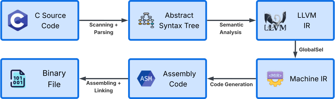
When a compiler takes the source code and produces a binary, it passes through several stages:

1. The scanner and parser take the raw source text and constructs an Abstract Syntax Tree (AST) to represent the program's grammar and meaning.

2. The AST is then lowered into an Intermediate Representation (IR), an architecture-neutral form that is easier to analyze and optimize.

   • LLVM Compiler Infrastructure makes a distinction between a high level IR (LLVM IR) and a low level IR (Machine IR)¹.

3. The Code Generator takes this IR and transforms it into assembly instructions for the target architecture.

4. The assembler translates the assembly instructions into binary machine code, producing an object fileA file of compiled machine code produced from source, before the linker combines it into a final executable. More →. The linker then combines these object files alongside any required libraries into a final executable binary.

Decompilation Pipeline

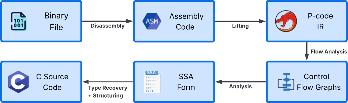
Like compilation, decompilation is not a single step but a pipeline of successive transformations, each building on the last. It traverses the same stages in reverse, starting from the binary and working backwards to reconstruct the original source code as faithfully as possible.

To build a decompiler, we need to understand what each stage does, what invariants it depends on, and where things can go wrong.

Dev's Note

This diagram shows a high-level view of the decompilation pipeline. The decompiler we will be building may not follow these stages exactly or in this exact order.

Disassembling through Recursive Descent

The first stage of decompilation aims to convert the raw machine code back into assembly instructions. By starting at a known entry point provided by the binary's header and recursively descending into all reachable branches, we can decode all the instructions contained in the binary to assembly instructions.

Consider the following fibonacci assembly pseudocode where we know the entry point of fibonacci at 0x1234.

0x1234 fibonacci:
    0x1234  CMP  n, 1          ; compare n to 1
    0x1238  JLE  0x1250        ; if n <= 1, jump to base case
    0x123c  CALL 0x1234        ; recursive call: fibonacci(n-1)
    0x1241  CALL 0x1234        ; recursive call: fibonacci(n-2)
    0x1246  ADD  result        ; add the two results
    0x124a  RET
    0x1250  MOV  eax, n        ; return n
    0x1254  RET

Starting at entry address 0x1234, the disassembler decodes instructions linearly until it hits a branch. At 0x1238, the conditional jump JLE has two possible branch paths: the fall-through at 0x123c and the target at 0x1250. The disassembler then descends into both paths, decoding instructions in each branch path until all reachable instructions have been visited.

Note

CALL 0x1234 instructions at 0x123c and 0x1241 resolve to the original address we already decoded. The disassembler will not descend into paths that lead to known addresses so that it does not repeat the disassembling process for the same path twice.

Once every branch has been followed, we now have completed the first stage of decompilation and recovered all the assembly instructions contained in the binary.

Adversarial reality check

This stage assumes the bytes you inspect are the bytes that matter. Packers, sandbox detection, self-modifying code, code/data overlap, and virtualization can all break that assumption before the decompiler really starts.

Converting to an Intermediate Representation (IR)

Now that we have the set of assembly instructions in hand, we need to lift these instructions into an IR, an architecture-neutral form of the program that removes the details of any specific ISAInstruction Set Architecture — the repertoire of instructions a CPU understands (e.g. x86-64, arm64, RISC-V). More →.

Consider this simple add_one function in C.

int add_one(int a) {
    return a + 1;
}

Here are the assembly instructions for this function in x86-64 and arm64.

x86-64:
0000000000001149 <add_one>:
    1149:       f3 0f 1e fa             endbr64 
    114d:       55                      push   %rbp
    114e:       48 89 e5                mov    %rsp,%rbp
    1151:       89 7d fc                mov    %edi,-0x4(%rbp)
    1154:       8b 45 fc                mov    -0x4(%rbp),%eax
    1157:       83 c0 01                add    $0x1,%eax
    115a:       5d                      pop    %rbp
    115b:       c3                      ret 

arm64:
0000000100000460 <_add_one>:
100000460: d10043ff     sub     sp, sp, #0x10
100000464: b9000fe0     str     w0, [sp, #0xc]
100000468: b9400fe8     ldr     w8, [sp, #0xc]
10000046c: 11000500     add     w0, w8, #0x1
100000470: 910043ff     add     sp, sp, #0x10
100000474: d65f03c0     ret

Even in a one line function, we can see that the majority of the instructions differ from each other. Common instructions like add have a different number of arguments and hex representations across ISAs. By lifting the assembly into an IR, we eliminate these architectural differences entirely. Throughout these blogs, we will be using Ghidra's p-codeGhidra's architecture-neutral intermediate representation for modelling what each instruction does. More → as our IR.

x86-64:
    ...
    CF = INT_CARRY EAX, 1:4
    OF = INT_SCARRY EAX, 1:4
    EAX = INT_ADD EAX, 1:4
    RAX = INT_ZEXT EAX
    SF = INT_SLESS EAX, 0:4
    ZF = INT_EQUAL EAX, 0:4
    ...
    RBP = COPY $Uaa400:8
    RIP = LOAD ram(RSP)
    RSP = INT_ADD RSP, 8:8
    RETURN RIP

arm64:
    ...
    tmpCY = INT_CARRY sp, $U23500:8
    tmpOV = INT_SCARRY sp, $U23500:8
    $U23700:8 = INT_ADD sp, $U23500:8
    tmpNG = INT_SLESS $U23700:8, 0:8
    tmpZR = INT_EQUAL $U23700:8, 0:8
    sp = COPY $U23700:8
    pc = COPY x30
    RETURN pc

Although the overall set of instructions still differs between architectures, each individual instruction now takes on a consistent form. This allows us to build a more uniform and manageable analyzer in the later stages, instead of a complex one that tries to handle every ISA separately.

Control Flow Graphs

The next stage is to organize these IR instructions into a Control Flow Graph (CFG). A CFG groups instructions into basic blocks, which are a sequence of instructions where only the last instruction can perform control flow, and connects them with edges that point to other reachable basic blocks.

For our fibonacci pseudocode above, there are three main basic blocks:

1. the condition check n <= 1

2. the base case

3. the recursive case

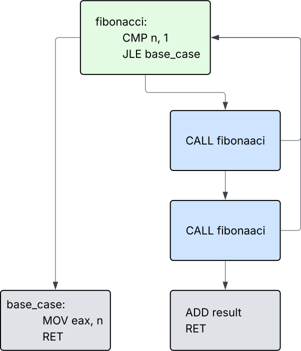
The CFG makes the overall flow of the program immediately apparent. Instead of manually tracing jump instructions, the CFG clarifies the overall flow of the program, helping us quickly understand when the program branches, recurses back, and ultimately terminates.

Converting the CFG into Static Single Assignment (SSA) Form

With the CFG in place, we need to convert the p-code IR into Static Single Assignment (SSA) form, which is another type of IR where each variable is assigned exactly once.

Consider the following code before SSA transformation:

x = 1
x = 2
y = x
y = y + x

When analyzing this code snippet, it may become confusing which values x and y hold at a given point. Such ambiguity in our IR may lead to difficulty in restructuring the C source code and produce inaccurate results.

Here is the same code in SSA form:

x_1 = 1
x_2 = 2
y_1 = x_2
y_2 = y_1 + x_2

After the transformation, it is much easier to understand which variables hold what values at every point in the program. SSA form provides a clear and unambiguous representation of data flow, making it easier to simplify redundant operations, track variable definitions, and ultimately reconstruct accurate variable names and types in the final C output.

Recovering the C source code

The last stage of the decompilation pipeline brings everything together. Using the CFG and SSA form, the decompiler can attempt to recover a readable C representation of the program through two closely related steps.

1) Type Recovery attempts to infer the types of variables from how they are used throughout the SSA form. For example, if a variable is used in a memory load with a 4-byte access, the decompiler can infer it is likely an int. If it is used as a pointer with an offset, it might be a struct or an array.

2) Structuring takes the CFG and attempts to reconstruct high-level control flow constructs, recovering if/else branches, for and while loops, and switch statements from what was previously just basic blocks and conditional jumps.

Here is a fully recovered C code from Ghidra:

int _add_one(int param_1)
{
  return param_1 + 1;
}

While the parameter name param_1 is a reminder that not everything survives compilation, we can see that the variable types, structure and logic of the function are fully intact.

Now that we have a sense of how the full pipeline works, we can start exploring the specific details of how each stage is actually implemented.

Content Review Quiz

Content Review Quiz

What is the main purpose of converting assembly instructions into an Intermediate Representation (IR)?

To compress the assembly into fewer number of instructions To create an architecture-neutral form that removes ISA-specific details To reduce the code execution time To make the instructions easier to read and understand

What is the defining rule of Static Single Assignment (SSA) form?

All assignments must occur at the start of the function Each variable can only be used once after it is assigned Assigned variables can never be modified Each variable is assigned exactly once

What is a key limitation of decompilation compared to the original source code?

It cannot determine which parts of the binary are actually executable code It cannot reliably reconstruct the exact original control structures used by the programmer It often loses high-level information like variable names and comments It cannot represent program logic in a high-level language

What is NOT a stage of the decompilation pipeline?

Disassembly of machine code into assembly Lifting instructions into an Intermediate Representation (IR) Converting IR into Static Single Assignment (SSA) form Generating optimized machine code for a target architecture

Check Answers

Try it yourself: tiny-dec

First, let's get your environment set up. We assume that you are running on Ubuntu/Debian.

Clone the Repository

$ git clone https://github.com/ZhangZhuoSJTU/tiny-dec
$ cd tiny-dec

Install Dependencies + Build Binaries

$ sudo apt-get install -y clang lld llvm binutils build-essential python3 python3-pip
$ pip install poetry
$ poetry install
$ ./scripts/build_fixtures.sh

Now that the environment is set up, let's take our decompiler for a spin!

Inspect the Binary

Before we decompile, let's peek inside the binary and see what we're working with. Pick any binary from ./tests/fixtures/bin and run:

$ poetry run tiny-dec info ./tests/fixtures/bin/fixture_basic_O0_nopie.elf 
binary: ./tests/fixtures/bin/fixture_basic_O0_nopie.elf
arch: riscv32 (32-bit, little-endian)
entrypoint: 0x110b4
entry_points: 0x110b4
main: 0x110b4
main_source: symbol_table
...
symbols:
  .Lline_table_start0              addr=0x0
  fixture_basic.c                  addr=0x0
  main                             addr=0x110b4
  helper                           addr=0x110f4
...

We can see some useful metadata such as the architecture, entrypoint address, and even the original function names main and helper preserved in the symbol tablea table in the binary that maps names, like function names, to their addresses.

Explore the Code: Decompile the Binary

Now for the exciting part — let's use our tiny-dec to turn this binary back into readable C code!

$ poetry run tiny-dec decompile ./tests/fixtures/bin/fixture_basic_O0_nopie.elf 
#include <stdint.h>
...
static ret_x10_x11 main(void) {
  int32_t local_12_4;
  struct { int32_t x10; uint32_t x11; } call_0x110d4_ret;

  local_12_4 = 7;
  call_0x110d4_ret = call_indirect_0x110f4(local_12_4);
  return (ret_x10_x11){.x10 = call_0x110d4_ret.x10 - 2, .x11 = call_0x110d4_ret.x11};
}

static ret_x10_x11 helper(int32_t arg_x10_4) {
  return (ret_x10_x11){.x10 = (arg_x10_4 << 1) + arg_x10_4 + 1, .x11 = arg_x10_4};
}

Compare this with the original source:

$ cat ./tests/fixtures/src/fixture_basic.c
#include <stdint.h>

static int helper(int x) {
    return x * 3 + 1;
}

int main(void) {
    int a = 7;
    int b = helper(a);
    return b - 2;
}

The resemblance is striking! Our decompiler successfully recovered both functions, their arguments, return values, and the core logic. The key difference is that low-level details like register names (x10, x11) and raw addresses appear in place of the clean variable names from the original. This is exactly the kind of information that gets lost during compilation and cannot be recovered, but the structure and logic of the program are fully intact.

What's Next?

In the next section, we will introduce the ISA we will be using on our decompiling journey and walk through the decoding stage, converting the hexadecimal machine code to the more readable assembly instructions.

Next chapter 1. Decoding Instructions

---

1. LLVM GlobalISel Pipeline ↩