Recursive Disassembly and Basic Blocks¶

Why is Disassembly Necessary?¶

By the end of post 2, every instruction can be lifted into p-codeGhidra's architecture-neutral intermediate representation for modelling what each instruction does. More →, giving us an architecture-independent description of its behavior. However, lifting alone only tells us what a single instruction does. It does not tell us which instructions belong to a function, where execution can continue, or how instructions should be grouped together for later analysis.

Consider the following code:

example_function:
    0x1000: addi x5, x0, 5
    0x1004: beq  x5, x0, 0x1010
    0x1008: addi x6, x0, 1
    0x100c: jal  x0, 0x1014
    0x1010: addi x6, x0, 2
    0x1014: ret

The lifter can translate each instruction into p-code independently, but it has no notion of execution flow. It does not know that:

execution begins at 0x1000
the branch at 0x1004 may continue to either 0x1008 or 0x1010
the jump at 0x100c skips over 0x1010
0x1014 can be reached from multiple paths

To answer these questions, we need disassembly. Disassembly determines which instructions belong to a function and how execution can flow between them. Once these relationships are known, later analyses such as data-flow, SSA construction, and control-flow structuring can operate on the program as a whole instead of isolated instructions.

Our decompiler uses recursive disassembly, but before discussing the algorithm, we first need to understand two fundamental concepts: basic blocks and control-flow graphs.

Basic Blocks¶

A basic block is a maximal sequence of instructions with a single entry and single exit point.

Basic blocks are constructed by decoding linearly from each discovered entry point until a control-flow boundary is reached.

A block ends when any of the following conditions is met:

a conditional branch is encountered
a direct jump is encountered
a return instruction is encountered
an indirect jump is encountered
a trap or invalid control-flow instruction is encountered
the next instruction address is already known to start another block

As each block is finalized, newly discovered successor addresses are added back into the worklist if they have not yet been processed.

Consider the following example RV32I function:

# example_func(int arg)
0x1000:  addi x5, x0, 0              # result = 0
0x1004:  beq  x10, x0, 0x102c        # if (arg == 0) go to done

loop:
0x1008:  jal  x1, helper_func        # direct call
0x100c:  add  x5, x5, x10            # result += arg
0x1010:  addi x10, x10, -1           # arg--
0x1014:  bne  x10, x0, 0x1008        # if (arg != 0) repeat ← back edge

0x1018:  jal  x0, 0x1024             # jump over inline data

0x101c:  .word 0xdeadbeef            # inline data
0x1020:  .word 0xcafebabe

0x1024:  lw   x6, 0(x11)             # load function pointer
0x1028:  jalr x0, 0(x6)              # indirect jump

done:
0x102c:  addi x10, x5, 0             # return value = result
0x1030:  ret

Applying the boundaries above to our running example gives five basic blocks:

Entry (0x1000-0x1004): initializes result and checks whether arg == 0. Ends at the conditional branch with two outgoing paths: one to done and one to the loop body.
Loop body (0x1008-0x1014): calls helper_func, accumulates the result, decrements arg, then tests whether arg has reached zero. If not, execution branches back to 0x1008, creating a back edge to the loop body itself. If so, execution falls through to 0x1018.
Data skip (0x1018): a single unconditional jump that skips over the two inline data words and lands at 0x1024.
Indirect jump (0x1024-0x1028): loads a function pointer and jumps to it. The destination is determined at runtime, so exploration stops here.
Done (0x102c-0x1030): copies the accumulated result into the return register and returns. Reached only when arg was initially zero.

Even though we now have structure at the instruction level, execution is still represented as a flat set of blocks. To reason about program behavior, we need to connect these blocks into a control-flow structure.

Control Flow Graphs¶

These blocks together form the nodes of a control-flow graph (CFG), where edges represent possible execution transfers between blocks.

While blocks are being formed, control-flow relationships are recorded at the same time:

conditional branches produce two outgoing edges: taken and fallthrough
direct jumps produce a single outgoing edge to the target
returns produce no outgoing edges
indirect jumps terminate the block but produce unresolved outgoing edges
calls are kept inside the block and recorded separately without affecting control flow

Applying these rules to the running example produces the following CFG:

Example CFG

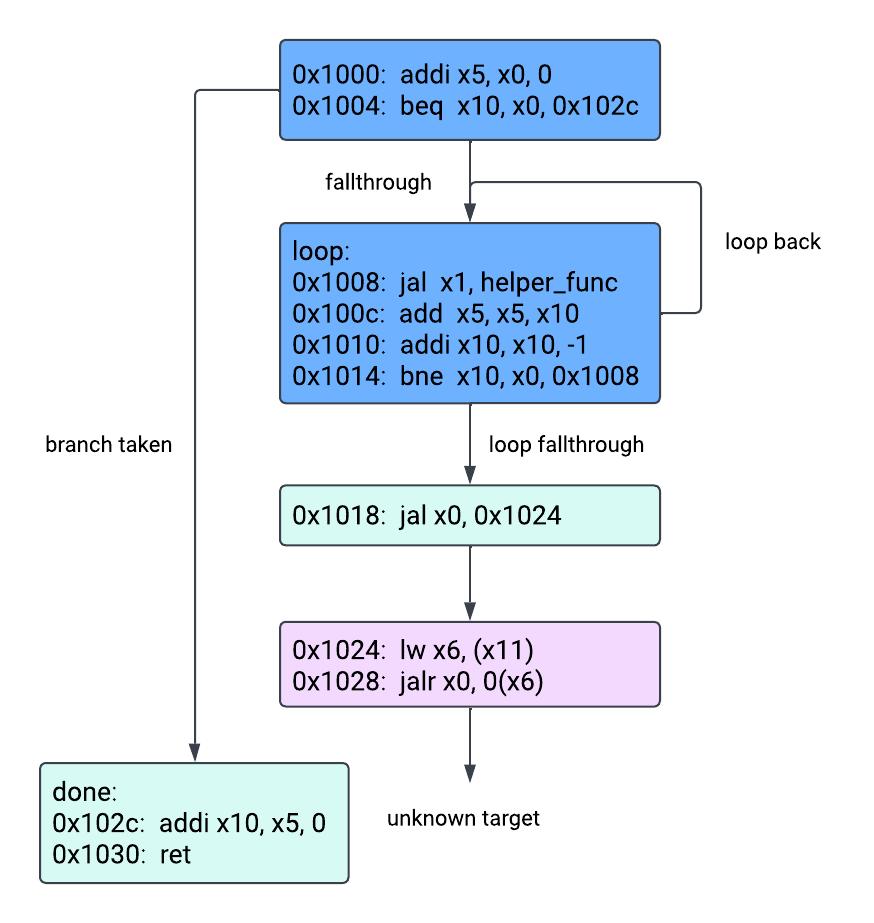
The entry block has two outgoing edges: one to the return block when arg == 0, and one to the loop body when execution falls through.

The loop body begins with a call to helper_func, updates result, decrements arg, and ends with the conditional branch at 0x1014. The branch has two outgoing edges: a back edge to the start of the loop when arg != 0, and a fallthrough edge to the unconditional jump block when the loop terminates. Although the block contains a call instruction, calls do not appear as CFG edges because execution resumes at the next instruction after the callee returns.

The unconditional jump block contains a single jal x0, 0x1024 instruction that skips over the inline data embedded in the code. Because its destination is known statically, it contributes a single outgoing edge to the indirect jump block.

The indirect jump block loads a destination address from memory and ends with jalr. Because the destination is determined at runtime rather than encoded in the instruction, the CFG records it as an unresolved edge instead of connecting it to a known successor.

Finally, the return block copies result into the return register and executes ret, producing no outgoing edges.

This CFG captures all statically known control flow in the function and provides the structural foundation for later analyses, such as data-flowhow values produced in one place get used elsewhere — the basis of later analysis stages tracking and higher-level reconstruction of the original program structure.

Linear Disassembly and its Limitations¶

The most direct way to disassemble a binary is to decode instructions strictly in address order, starting at the beginning of a code section and continuing one instruction at a time until the section ends. This is linear disassembly.

Linear disassembly works well as long as every byte in the region being decoded is actually an instruction. While this assumption holds for large stretches of real programs, it breaks down whenever non-code bytes are interleaved with code.

When linear disassembly comes across inline dataliteral constants or raw data embedded directly within the sequence of machine instructions., it has no way to distinguish it from an instruction. It decodes the bytes anyway, producing an instruction that does not actually exist within the program. Decoding can then potentially drift out of alignment for subsequent instructions, producing instructions that significantly differ from the original program's behavior.

Consider the inline data in our running example:

0x1018:  jal  x0, 0x1024

0x101c:  .word 0xdeadbeef 
0x1020:  .word 0xcafebabe

0x1024:

A linear disassembler would continue decoding after the jal x0, 0x1024 instruction and attempt to interpret the two .word values at 0x101c and 0x1020 as RV32I instructions. Because these bytes are actually embedded data, the resulting instructions would be meaningless and could even cause subsequent decoding to become misaligned. Although execution can never reach these bytes, a linear disassembler has no way to distinguish them from code.

This is the central limitation of linear disassembly: it has no notion of reachability. By disassembling linearly, it commits to every byte in a region being code, with no way to recognize data sitting in the middle of it.

Recursive Disassembly¶

Where linear disassembly commits to decoding every byte in a region, recursive disassembly starts from a known entry address and decodes only code that can be determined to be reachable.

The process begins at the function entry address and decodes instructions linearly. When a control-flow instruction is encountered, decoding does not continue blindly. Instead, the disassembler extracts the possible successor addresses and treats them as new points of exploration.

The discovered successor addresses are placed into a worklist. Each address in the worklist represents a potential entry into previously unseen code. The disassembler repeatedly processes this worklist until no new reachable addresses remain.

During this exploration, control-flow instructions are handled as follows:

conditional branches contribute two successors: the branch target and the fallthrough path
direct jumps contribute a single successor to the target address
direct calls record the callee as another function entry and continue execution at the fallthrough address without any new successors
returns terminate the current path

Like any static analysis technique, however, recursive disassembly is not perfect. Some control-flow targets cannot be determined statically. Indirect jumps, jump tables, dynamically computed branch targets, and certain forms of obfuscationDeliberately transforming code to make it hard to analyze or reverse-engineer, while preserving what it does. More → can all prevent the disassembler from discovering every reachable block. When no concrete destination can be resolved, exploration must stop at that point until later analysis or additional information becomes available.

In our example, when execution reaches 0x1028: jalr x0, 0(x6), the destination depends on the runtime value stored in x6. Without additional analysis, the disassembler cannot determine where execution will continue, so exploration stops at this block. Later analyses, such as constant propagation, value tracking, or jump-table recovery, may resolve the destination, but recursive disassembly alone cannot.

Nevertheless, most compiled programs spend the majority of their execution following direct branches, direct jumps, and direct function calls, all of which recursive disassembly handles effectively. By focusing only on reachable code, recursive disassembly produces an accurate structural view of a function while avoiding many of the pitfalls of linear disassembly.

Content Review Quiz¶

Explore the Code¶

Let's take a look at the tiny-dec disassembly code to understand how the p-code instructions are structured to form basic blocks and create a control-flow graph.

Code Structure¶

models.py contains the dataclasses needed to structure the instructions into basic blocks and output the fully disassembled result from this stage.

BasicBlock is the dataclass that groups RV32IInstruction objects from the previous decoding stage into basic blocks and connects them into a control-flow graph by maintaining BlockEdge objects pointing to their successors:

start: the entry address for the block
instructions: a list of BlockInstruction, which pairs each RV32IInstruction with its p-code ops, contained in this block
successors: a list of outgoing edges to other basic blocks that are successors of this block
terminator: how the current basic block terminated

DisasmFunction is the final output of this stage that tracks BasicBlocks found during disassembly.

Code Walkthrough¶

The core functionality of the disassembler lies in the function disassemble_function in builder.py, which builds the DisasmFunction output in four steps.

Step 1: Start from a Known Entry Address. disassemble_function starts with the function entry as the only known block leader. That address is also placed into the worklist and marked as scheduled so it is not queued more than once.

known_leaders = {entry}
scheduled = {entry}
worklist = [entry]

Step 2: Decode the block linearly. An address is popped from the worklist and passed to _decode_block, which repeatedly decodes and lifts instructions until a block boundary is reached.

while worklist:
    block_start = worklist.pop()
    ...
    block = _decode_block(..., block_start, ...)

def _decode_block(...):
    while True:
        ...
        instruction = decode_rv32i(word, address)
        lifted = BlockInstruction(
            instruction=instruction,
            pcode_ops=tuple(lift_instruction(instruction)),
        )
        instructions.append(lifted)
        ...

Step 3: Terminate the Block. To determine if a block should be terminated, _decode_block calls _classify_terminator on each lifted instruction.

When _classify_terminator identifies a terminating instruction, _decode_block finalizes the current BasicBlock, records its terminator and successor edges, and returns it. The discovered successors are then available for disassemble_function to schedule for exploration.

Step 4: Drain the worklist. The successors of the returned basic block are added to the worklist, and steps 2–4 repeat from each new address until the worklist is empty.

while worklist:
    block_start = worklist.pop()
    ...
    block = _decode_block(view, block_start, known_leaders)
    ...
    for successor in reversed(block.successors):
        if successor.target in scheduled:
            continue
        worklist.append(successor.target)

Let's run tiny-dec's disassembly stage on the mix function from fixture_chain.c to see how the stage handles a function with multiple blocks.

static int mix(int left, int right) {
    if (left < right) {
        return bump(left + right);
    }
    return bump(left - right);
}

$ poetry run tiny-dec decompile ./tests/fixtures/bin/fixture_chain_O0_nopie.elf --stage disasm --func mix
...
disasm:
  entry: 0x111b4
  order: 0x111b4, 0x111f4, 0x1120c, 0x111d8, 0x111dc
  block 0x111b4 term=branch succ=[branch_taken:0x111f4, fallthrough:0x111d8]
    ...
    0x000111d4: 0x02b55063  bge x10, x11, 0x111f4
      INT_SLESS unique[0x0:1] <- register[0xa:4], register[0xb:4]
      BOOL_NEGATE unique[0x4:1] <- unique[0x0:1]
      CBRANCH const[0x111f4:4], unique[0x4:1]
  block 0x111f4 term=jump succ=[jump:0x1120c] calls=[0x11220]
    ...
  block 0x1120c term=return succ=[]
    ...
  block 0x111d8 term=jump succ=[jump:0x111dc]
    ...
  block 0x111dc term=jump succ=[jump:0x1120c] calls=[0x11220]
    ...

Step 1 seeds the worklist with {0x111b4}.

Step 2 decodes from 0x111b4 linearly until 0x111d4, where bge x10, x11, 0x111f4 lifts to a CBRANCH op.

Step 3 closes block 0x111b4 with term=branch and two successors: branch_taken:0x111f4 and fallthrough:0x111d8.

Step 4 pushes the successors onto the worklist in reversed order (0x111d8 first, then 0x111f4), so 0x111f4 is popped next.

The same process repeats until the worklist is empty:

0x111f4: decodes linearly, hits jal x0, 0x1120c (a direct jump), closes with term=jump succ=[jump:0x1120c], adding 0x1120c to the worklist.
0x1120c: decodes linearly, hits jalr x0, 0(x1) (a return), closes with term=return succ=[], therefore not adding anything to the worklist.
0x111d8: a single jal x0, 0x111dc instruction, closes with term=jump succ=[jump:0x111dc], adding 0x111dc to the worklist.
0x111dc: decodes linearly, hits jal x0, 0x1120c (a direct jump), closes with term=jump succ=[jump:0x1120c]. 0x1120c has already been discovered, so nothing is added.

Once the worklist is empty, every reachable block has been discovered and disassemble_function returns the DisasmFunction containing the five recovered blocks in discovery_order: (0x111b4, 0x111f4, 0x1120c, 0x111d8, 0x111dc).

Notice that: 1. 0x1120c appears in discovery_order before 0x111d8 and 0x111dc. This is a consequence of the LIFO worklist: 0x111f4 was pushed last and popped first, discovering 0x1120c before the fallthrough path was ever explored. The discovery order reflects traversal order, not address order. 2. No unreachable addresses are ever decoded. Every new block begins because it was reached through a successor edge from a previously discovered block, illustrating the key idea behind recursive disassembly.

What's Next?¶

The next step is to turn these basic blocks into durable, typed containers that subsequent stages can consume without needing to rediscover function-level structure from raw bytes.

Additional Readings¶

If you would like to learn more, these papers explore disassembly techniques and obfuscation, as well as reassemblers and the challenges of converting machine code back into compilable source code or even assembly code.